Competition : https://www.kaggle.com/c/bike-sharing-demand/overview
Code : https://www.kaggle.com/viveksrinivasan/eda-ensemble-model-top-10-percentile
Description

1. About Dataset
- datetime : hourly date + timestamp
- season : 1 = spring, 2 = summer, 3 = fall, 4 = winter
- holiday : whether the day is considered a holiday
- workingday : whether the day is neither a weekend nor holiday
- weather :
- 1: Clear, Few clouds, Partly cloudy, Partly cloudy
- 2: Mist + Cloudy, Mist + Broken clouds, Mist + Few clouds, Mist
- 3: Light Snow, Light Rain + Thunderstorm + Scattered clouds, Light Rain + Scattered clouds
- 4: Heavy Rain + Ice Pallets + Thunderstorm + Mist, Snow + Fog
- temp : temperature in Celsius
- atemp : "feels like" temperature in Celsius
- humidity : relative humidity
- windspeed : wind speed
- casual : number of non-registered user rentals initiated
- registered : number of registered user rentals initiated
- count : number of total rentals
Package Load
import pylab
import calendar
import numpy as np
import pandas as pd
import seaborn as sn
from scipy import stats
import missingno as msno
from datetime import datetime
import matplotlib.pyplot as plt
import warnings
pd.options.mode.chained_assignment = None
warnings.filterwarnings("ignore", category=DeprecationWarning)
%matplotlib inline
2. Data Summary
Shape Of The Dataset
dailyData.shape

>>>
(10886, 12)
Sample of First Few Rows
Data Type
3. Feature Engineering
위 변수중 season, holiday, workingday, weather는 categorical 변수여야 하지만 데이터 타입이 integer로 되어있다.
- datetime column에서 date, hour, weekday, month column을 새롭게 생성한다.
- season, holiday, workingday, weather를 categorical로 변경해준다. (각 변수들에서 추출한 변수들도 마찬가지)
- 새로운 변수를 추출하기 위해 사용한 column은 삭제해준다.
1. Creating New Columns From Datetime Column
dailyData["date"] = dailyData.datetime.apply(lambda x : x.split()[0])
dailyData["hour"] = dailyData.datetime.apply(lambda x : x.split()[1].split(":")[0])
dailyData["weekday"] = dailyData.date.apply(lambda dateString : calendar.day_name[datetime.strptime(dateString,"%Y-%m-%d").weekday()])
dailyData["month"] = dailyData.date.apply(lambda dateString : calendar.month_name[datetime.strptime(dateString,"%Y-%m-%d").month])
dailyData["season"] = dailyData.season.map({1: "Spring", 2 : "Summer", 3 : "Fall", 4 :"Winter" })
dailyData["weather"] = dailyData.weather.map({1: " Clear + Few clouds + Partly cloudy + Partly cloudy",\
                                        2 : " Mist + Cloudy, Mist + Broken clouds, Mist + Few clouds, Mist ", \
                                        3 : " Light Snow, Light Rain + Thunderstorm + Scattered clouds, Light Rain + Scattered clouds", \
                                        4 :" Heavy Rain + Ice Pallets + Thunderstorm + Mist, Snow + Fog " })
2. Coercing To Category Type
categoryVariableList = ["hour","weekday","month","season","weather","holiday","workingday"]
for var in categoryVariableList:
    dailyData[var] = dailyData[var].astype("category")
3. Dropping Unnecessary Columns
dailyData = dailyData.drop(["datetime"],axis=1)데이터 타입별 변수 갯수 count
dataTypeDf = pd.DataFrame(dailyData.dtypes.value_counts()).reset_index().rename(columns={"index":"variableType",0:"count"})
fig,ax = plt.subplots()
fig.set_size_inches(12,5)
sn.barplot(data=dataTypeDf,x="variableType",y="count",ax=ax)
ax.set(xlabel='variableTypeariable Type', ylabel='Count',title="Variables DataType Count")
앞서 생성 및 변환한 변수 중 date를 제외하고 모두 category로 변환. date는 object type
4. Missing Values Analysis
missingno library를 이용하여 데이터셋의 결측치 확인
msno.matrix(dailyData,figsize=(12,5))5. Outliers Analysis
fig, axes = plt.subplots(nrows=2,ncols=2)
fig.set_size_inches(12, 10)
sn.boxplot(data=dailyData,y="count",orient="v",ax=axes[0][0])
sn.boxplot(data=dailyData,y="count",x="season",orient="v",ax=axes[0][1])
sn.boxplot(data=dailyData,y="count",x="hour",orient="v",ax=axes[1][0])
sn.boxplot(data=dailyData,y="count",x="workingday",orient="v",ax=axes[1][1])

axes[0][0].set(ylabel='Count',title="Box Plot On Count")
axes[0][1].set(xlabel='Season', ylabel='Count',title="Box Plot On Count Across Season")
axes[1][0].set(xlabel='Hour Of The Day', ylabel='Count',title="Box Plot On Count Across Hour Of The Day")
axes[1][1].set(xlabel='Working Day', ylabel='Count',title="Box Plot On Count Across Working Day")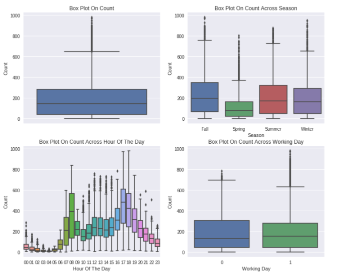
- Count 변수를 봤을 때, Right-skewed를 보이면서 많은 outlier data를 가지고 있다.
- Spring season에는 상대적으로 낮은 count를 보인다. 이는 boxplot의 median value가 매우 낮은 것으로 확인할 수 있다.
- Hour of the day 변수를 보면 오전 7~8시, 오후 5~6시에 높은 값을 보이는데, 이는 학교와 직장과 관련이 있는 것으로 보인다.
- 대부분의 outlier는 'Non Working Day' 보다 'Working Day'에 존재한다.
Remove Outliers in The Count Column
dailyDataWithoutOutliers = dailyData[np.abs(dailyData["count"]-
		dailyData["count"].mean())<=(3*dailyData["count"].std())]

print ("Shape Of The Before Ouliers: ",dailyData.shape)
print ("Shape Of The After Ouliers: ",dailyDataWithoutOutliers.shape)

>>>
Shape Of The Before Ouliers:  (10886, 15)
Shape Of The After Ouliers:  (10739, 15)
6. Correlation Analysis
종속 변수가 feature에 의해 영향을 받는 방식을 이해하는 일반적인 방법은 이들간의 상관 행렬을 fibd 하는 것입니다.
- fibd : 데이터 세트에 있는 모든 고유 BD 모드의 FI(failure intensity)를 계산하는 테이블을 작성. 이는 Crow Extended 또는 Crow Extended - 연속 평가 모델로 분석된 데이터 세트에만 적용됩니다.
corrMatt = dailyData[["temp","atemp","casual","registered","humidity","windspeed","count"]].corr()
mask = np.array(corrMatt)
mask[np.tril_indices_from(mask)] = False
fig,ax= plt.subplots()
fig.set_size_inches(20,10)
sn.heatmap(corrMatt, mask=mask,vmax=.8, square=True,annot=True)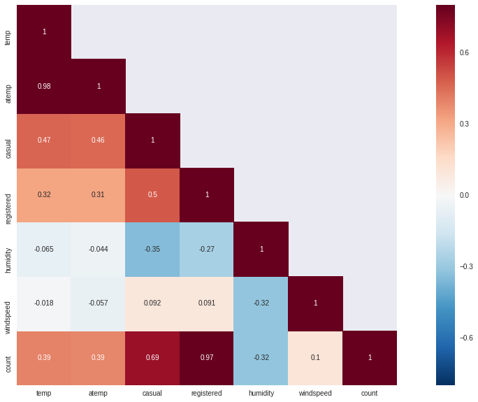
- temp와 humidity는 count와 각각 양(0.39), 음(-0.32)의 상관관계를 가진다. 이들간의 상관관계를 count가 변수들에 대해 약한 의존성을 가지고 있기 때문에 매우 중요하지는 않다.
- windspeed는 count와의 상관관계를 봤을 때, 쓸모있는 변수는 아니다.
- atemp변수는 temp와 0.98의 상관관계를 가지기 때문에 제거한다. model building을 하는 과정에서 다중공선성을 가지는 변수는 반드시 제거해야 한다.
- 다중공선성 : 통계학의 회귀분석에서 독립변수들 간에 강한 상관관계가 나타나는 문제이다.
- casual과 registered는 본질적으로 leakage variables인데, 이는 모델 구축 중에 삭제해야 하기 때문에 고려되지 않습니다.
fig,(ax1,ax2,ax3) = plt.subplots(ncols=3)
fig.set_size_inches(12, 5)
sn.regplot(x="temp", y="count", data=dailyData,ax=ax1)
sn.regplot(x="windspeed", y="count", data=dailyData,ax=ax2)
sn.regplot(x="humidity", y="count", data=dailyData,ax=ax3)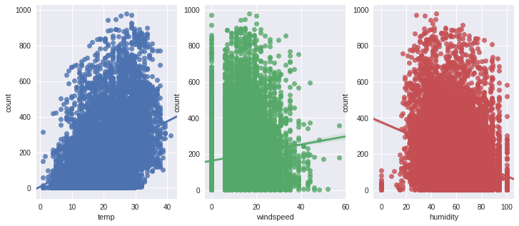
7. Visualizing Distribution of Data
fig,axes = plt.subplots(ncols=2,nrows=2)
fig.set_size_inches(12, 10)
sn.distplot(dailyData["count"],ax=axes[0][0])
stats.probplot(dailyData["count"], dist='norm', fit=True, plot=axes[0][1])
sn.distplot(np.log(dailyDataWithoutOutliers["count"]),ax=axes[1][0])
stats.probplot(np.log1p(dailyDataWithoutOutliers["count"]), dist='norm', fit=True, plot=axes[1][1])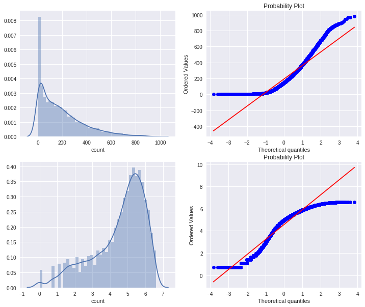
count 변수에 대한 정규성을 확인해 본 결과 Right-skewed한 모양을 가지고 있다. 대부분의 머신 러닝 기술은 종속 변수가 Normal이어야 하므로 정규 분포를 갖는 것이 바람직하다. 이를 해결하기 위한 방법중 하나는 이상치를 제거한 변수에 대해 log변환을 진행하는 것인데, 변환을 진행한 결과 좀 나아보이지만 여전히 정규분포를 따르지는 않는다.
8. Visualizing Count Vs (Month, Season, Hour, Weekday, Usertype)
fig,(ax1,ax2,ax3,ax4)= plt.subplots(nrows=4)
fig.set_size_inches(12,20)
sortOrder = ["January","February","March","April","May","June","July","August","September","October","November","December"]
hueOrder = ["Sunday","Monday","Tuesday","Wednesday","Thursday","Friday","Saturday"]
monthAggregated = pd.DataFrame(dailyData.groupby("month")["count"].mean()).reset_index()
monthSorted = monthAggregated.sort_values(by="count",ascending=False)
sn.barplot(data=monthSorted,x="month",y="count",ax=ax1,order=sortOrder)
ax1.set(xlabel='Month', ylabel='Avearage Count',title="Average Count By Month")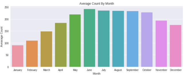
여름 시즌에 자전거를 타기에 정말 좋은 계절이기 때문에 사람들이 자전거를 빌리는 경향이 있다는 것은 분명합니다. 따라서 6월, 7월, 8월에는 자전거 수요가 상대적으로 높습니다.
hourAggregated = pd.DataFrame(dailyData.groupby(["hour","season"],sort=True)["count"].mean()).reset_index()
sn.pointplot(x=hourAggregated["hour"], y=hourAggregated["count"],hue=hourAggregated["season"], data=hourAggregated, join=True,ax=ax2)
ax2.set(xlabel='Hour Of The Day', ylabel='Users Count',title="Average Users Count By Hour Of The Day Across Season",label='big')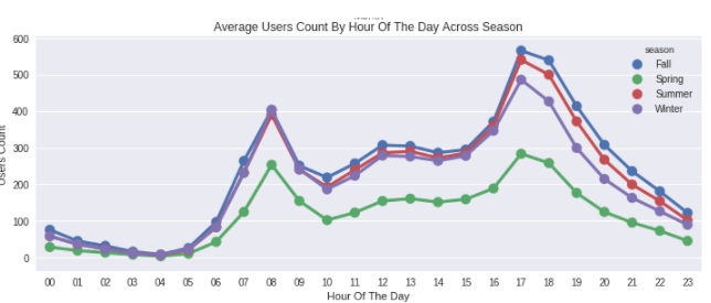
평일 오전 7시~오전 8시, 오후 5시~6시 사이에 자전거를 빌리는 사람들이 더 많습니다. 앞서 언급했듯이 이것은 일반 학교 및 사무실 통근자들의 영향일 수 있습니다.
hourAggregated = pd.DataFrame(dailyData.groupby(["hour","weekday"],sort=True)["count"].mean()).reset_index()
sn.pointplot(x=hourAggregated["hour"], y=hourAggregated["count"],hue=hourAggregated["weekday"],hue_order=hueOrder, data=hourAggregated, join=True,ax=ax3)
ax3.set(xlabel='Hour Of The Day', ylabel='Users Count',title="Average Users Count By Hour Of The Day Across Weekdays",label='big')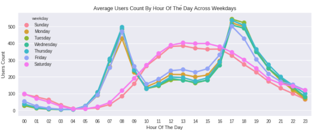
위의 패턴은 토요일과 일요일에는 맞지 않습니다. 사람들은 오전10시~오후4시 사이에 많이 빌리는 경향을 보입니다.
hourTransformed = pd.melt(dailyData[["hour","casual","registered"]], id_vars=['hour'], value_vars=['casual', 'registered'])
hourAggregated = pd.DataFrame(hourTransformed.groupby(["hour","variable"],sort=True)["value"].mean()).reset_index()
sn.pointplot(x=hourAggregated["hour"], y=hourAggregated["value"],hue=hourAggregated["variable"],hue_order=["casual","registered"], data=hourAggregated, join=True,ax=ax4)
ax4.set(xlabel='Hour Of The Day', ylabel='Users Count',title="Average Users Count By Hour Of The Day Across User Type",label='big')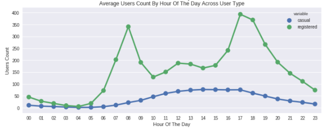
오전 7~8시와 오후 5~6시에 가장 높은 count를 보이는 것은 registered user에 영향을 많이 받았다.
9. Filling 0's In windspeed Using Random Forest
windspeed가 0인 부분을 결측치로 판단하고, 이부분을 예측을 통해 결측치 처리
dataTrain = pd.read_csv("../input/train.csv")
dataTest = pd.read_csv("../input/test.csv")

data = dataTrain.append(dataTest)
data.reset_index(inplace=True)
data.drop('index',inplace=True,axis=1)

#Feature Engineering
data["date"] = data.datetime.apply(lambda x : x.split()[0])
data["hour"] = data.datetime.apply(lambda x : x.split()[1].split(":")[0]).astype("int")
data["year"] = data.datetime.apply(lambda x : x.split()[0].split("-")[0])
data["weekday"] = data.date.apply(lambda dateString : datetime.strptime(dateString,"%Y-%m-%d").weekday())
data["month"] = data.date.apply(lambda dateString : datetime.strptime(dateString,"%Y-%m-%d").month)
Random Forest Model To Predict 0's In Windspeed
from sklearn.ensemble import RandomForestRegressor

dataWind0 = data[data["windspeed"]==0]
dataWindNot0 = data[data["windspeed"]!=0]
rfModel_wind = RandomForestRegressor()
windColumns = ["season","weather","humidity","month","temp","year","atemp"]
rfModel_wind.fit(dataWindNot0[windColumns], dataWindNot0["windspeed"])

wind0Values = rfModel_wind.predict(X= dataWind0[windColumns])
dataWind0["windspeed"] = wind0Values
data = dataWindNot0.append(dataWind0)
data.reset_index(inplace=True)
data.drop('index',inplace=True,axis=1)Coercing To Categorical Type
categoricalFeatureNames = ["season","holiday","workingday","weather","weekday","month","year","hour"]
numericalFeatureNames = ["temp","humidity","windspeed","atemp"]
dropFeatures = ['casual',"count","datetime","date","registered"]

for var in categoricalFeatureNames:
    data[var] = data[var].astype("category")
Splitting Train And Test Data, Dropping Unncessary Variables
dataTrain = data[pd.notnull(data['count'])].sort_values(by=["datetime"])
dataTest = data[~pd.notnull(data['count'])].sort_values(by=["datetime"])
#앞에서 train과 test 데이터를 합쳐서 진행했기 때문에, count 유무로 다시 나눔
datetimecol = dataTest["datetime"]
yLabels = dataTrain["count"]
yLablesRegistered = dataTrain["registered"]
yLablesCasual = dataTrain["casual"]

dataTrain  = dataTrain.drop(dropFeatures,axis=1)
dataTest  = dataTest.drop(dropFeatures,axis=1)
10. Modeling
Define RMSLE
def rmsle(y, y_,convertExp=True):
    if convertExp:
        y = np.exp(y),
        y_ = np.exp(y_)
    log1 = np.nan_to_num(np.array([np.log(v + 1) for v in y]))
    log2 = np.nan_to_num(np.array([np.log(v + 1) for v in y_]))
    calc = (log1 - log2) ** 2
    return np.sqrt(np.mean(calc))
Linear Regression Model
from sklearn.linear_model import LinearRegression,Ridge,Lasso
from sklearn.model_selection import GridSearchCV
from sklearn import metrics
import warnings
pd.options.mode.chained_assignment = None
warnings.filterwarnings("ignore", category=DeprecationWarning)

# Initialize logistic regression model
lModel = LinearRegression()

# Train the model
yLabelsLog = np.log1p(yLabels)
lModel.fit(X = dataTrain,y = yLabelsLog)

# Make predictions
preds = lModel.predict(X= dataTrain)
print ("RMSLE Value For Linear Regression: ",rmsle(np.exp(yLabelsLog),np.exp(preds),False))

>>>
RMSLE Value For Linear Regression:  0.977995978355
Regularization Model - Ridge
ridge_m_ = Ridge()
ridge_params_ = { 'max_iter':[3000],'alpha':[0.1, 1, 2, 3, 4, 10, 30,100,200,300,400,800,900,1000]}
rmsle_scorer = metrics.make_scorer(rmsle, greater_is_better=False)
grid_ridge_m = GridSearchCV( ridge_m_,
                          ridge_params_,
                          scoring = rmsle_scorer,
                          cv=5)
yLabelsLog = np.log1p(yLabels)
grid_ridge_m.fit( dataTrain, yLabelsLog )
preds = grid_ridge_m.predict(X= dataTrain)
print (grid_ridge_m.best_params_)
print ("RMSLE Value For Ridge Regression: ",rmsle(np.exp(yLabelsLog),np.exp(preds),False))

fig,ax= plt.subplots()
fig.set_size_inches(12,5)
df = pd.DataFrame(grid_ridge_m.grid_scores_)
df["alpha"] = df["parameters"].apply(lambda x:x["alpha"])
df["rmsle"] = df["mean_validation_score"].apply(lambda x:-x)
sn.pointplot(data=df,x="alpha",y="rmsle",ax=ax)

>>>
{'alpha': 0.1, 'max_iter': 3000}
RMSLE Value For Ridge Regression:  0.97799596327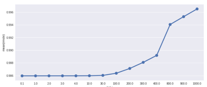
- make_scorer의 custom_scoring : custom scoring 함수
- make_scorer의 greater_is_better : False는 score 값이 낮은게 좋음을 의미
Regularization Model - Lasso
lasso_m_ = Lasso()

alpha  = 1/np.array([0.1, 1, 2, 3, 4, 10, 30,100,200,300,400,800,900,1000])
lasso_params_ = { 'max_iter':[3000],'alpha':alpha}

grid_lasso_m = GridSearchCV( lasso_m_,lasso_params_,scoring = rmsle_scorer,cv=5)
yLabelsLog = np.log1p(yLabels)
grid_lasso_m.fit( dataTrain, yLabelsLog )
preds = grid_lasso_m.predict(X= dataTrain)
print (grid_lasso_m.best_params_)
print ("RMSLE Value For Lasso Regression: ",rmsle(np.exp(yLabelsLog),np.exp(preds),False))

fig,ax= plt.subplots()
fig.set_size_inches(12,5)
df = pd.DataFrame(grid_lasso_m.grid_scores_)
df["alpha"] = df["parameters"].apply(lambda x:x["alpha"])
df["rmsle"] = df["mean_validation_score"].apply(lambda x:-x)
sn.pointplot(data=df,x="alpha",y="rmsle",ax=ax)

>>>
{'alpha': 0.0050000000000000001, 'max_iter': 3000}
RMSLE Value For Lasso Regression:  0.978133604313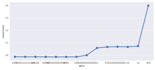
Ensemble Models - Random Forest
from sklearn.ensemble import RandomForestRegressor
rfModel = RandomForestRegressor(n_estimators=100)
yLabelsLog = np.log1p(yLabels)
rfModel.fit(dataTrain,yLabelsLog)
preds = rfModel.predict(X= dataTrain)
print ("RMSLE Value For Random Forest: ",rmsle(np.exp(yLabelsLog),np.exp(preds),False))

>>>
RMSLE Value For Random Forest:  0.102804484141
Ensemble Models - Gradient Boost
from sklearn.ensemble import GradientBoostingRegressor
gbm = GradientBoostingRegressor(n_estimators=4000,alpha=0.01); ### Test 0.41
yLabelsLog = np.log1p(yLabels)
gbm.fit(dataTrain,yLabelsLog)
preds = gbm.predict(X= dataTrain)
print ("RMSLE Value For Gradient Boost: ",rmsle(np.exp(yLabelsLog),np.exp(preds),False))

>>>
RMSLE Value For Gradient Boost:  0.189973542608
predsTest = gbm.predict(X= dataTest)
fig,(ax1,ax2)= plt.subplots(ncols=2)
fig.set_size_inches(12,5)
sn.distplot(yLabels,ax=ax1,bins=50)
sn.distplot(np.exp(predsTest),ax=ax2,bins=50)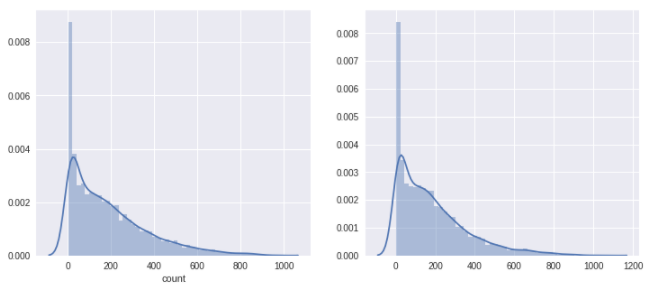
학습 데이터와 테스트 결과를의 분포를 비교해 본 결과, 비슷한 분포를 보이는 것을 확인할 수 있는데 이는 모델이 실제로 예측을 나쁘지 않게 했고, Overfitting 문제로 겪지 않았음을 확인할 수 있다.
The submission will have test score of 0.41
참고 문헌
https://ko.wikipedia.org/wiki/%EB%8B%A4%EC%A4%91%EA%B3%B5%EC%84%A0%EC%84%B1
'Kaggle' 카테고리의 다른 글
| New York City Taxi Trip Duration 코드리뷰 (0) | 2022.02.01 |
|---|---|
| House Prices - Advanced Regression Techniques 코드리뷰 2 (0) | 2022.01.26 |
| House Prices - Advanced Regression Techniques 코드리뷰 (0) | 2022.01.17 |


댓글